###############tensorflow实现 风格迁移 实例################
原理之前介绍过,这里只介绍实现:
基于 VGG19 定义自己的图像特征提取NN网络模型: 从预训练的模型中,获取卷积层部分的参数,用于构建我们自己的模型。VGG19中的全连接层舍弃掉,这一部分对提取图像特征基本无用。
这里提取出来的VGG参数全部是作为constant(即常量)使用的,也就是说,这些参数是不会再被训练的,在反向传播的过程中也不会改变。
另外,输入层要设置为Variable,我们要训练的就是这个变量;
最开始输入一张噪音图片,然后不断地根据内容loss和风格loss对其进行调整,直到一定次数后,该图片兼具了风格图片的风格以及内容图片的内容。当训练结束时,输入层的参数就是我们生成的图片。
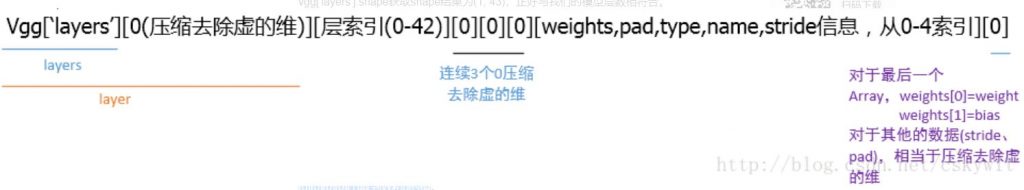
由于我们读取的模型为imagenet-vgg-verydeep-19.mat 模型文件,其参数存储结构影响到我们如何取w和b的值,如下:
开始模型训练:
先定义模型训练需要的一些参数:
STYLE = 'guernica'
CONTENT = 'deadpool'
STYLE_IMAGE = 'styles/' + STYLE + '.jpg'
CONTENT_IMAGE = 'content/' + CONTENT + '.jpg'
IMAGE_HEIGHT = 250
IMAGE_WIDTH = 333
NOISE_RATIO = 0.6

CONTENT_WEIGHT = 0.01
STYLE_WEIGHT = 1

# 在VGG的Layers中选择部分作为风格特征提取层
STYLE_LAYERS = ['conv1_1', 'conv2_1', 'conv3_1', 'conv4_1', 'conv5_1']
#针对上面各layer的风格特征的权重
STYLE_LAYERS_W = [0.5, 1.0, 1.5, 3.0, 4.0]  # give more weights to deeper layers.

#   在VGG的Layers中选择部分作为内容特征提取层,可自行修改
CONTENT_LAYER = 'conv4_2'
#迭代次数
ITERS = 300
#梯度下降学习率
LR = 2.0

#为了对输入图片预处理,归一化处理(通过图片像素减去均值),定义的均值像素
MEAN_PIXELS = np.array([123.68, 116.779, 103.939]).reshape((1, 1, 1, 3))


# VGG-19参数文件URL 和名字
VGG_DOWNLOAD_LINK = 'http://www.vlfeat.org/matconvnet/models/imagenet-vgg-verydeep-19.mat'
VGG_MODEL = 'imagenet-vgg-verydeep-19.mat'

EXPECTED_BYTES = 534904783
总体训练流程主函数:
def main():
    with tf.variable_scope('input') as scope:
        #定义input tensor为一个变量(而不是placeholder),因为它是被训练的对象
        input_image = tf.Variable(np.zeros([1, IMAGE_HEIGHT, IMAGE_WIDTH, 3]), dtype=tf.float32)

    #加载预训练VGG模型参数
    utils.download(VGG_DOWNLOAD_LINK, VGG_MODEL, EXPECTED_BYTES)
    utils.make_dir('checkpoints')
    utils.make_dir('outputs')
    model = vgg_model(VGG_MODEL, input_image)

    #设置变量global_step(训练过程中值会变化),保存到model['global_step']中
    model['global_step'] = tf.Variable(0, dtype=tf.int32, trainable=False, name='global_step')

    #加载内容图片和风格图片,预处理(resize,归一化)
    content_image = utils.get_resized_image(CONTENT_IMAGE, IMAGE_HEIGHT, IMAGE_WIDTH)
    content_image = content_image - MEAN_PIXELS
    style_image = utils.get_resized_image(STYLE_IMAGE, IMAGE_HEIGHT, IMAGE_WIDTH)
    style_image = style_image - MEAN_PIXELS

    #计算的损失值保存在model的字典中
    model['content_loss'], model['style_loss'], model['total_loss'] = _create_losses(model, input_image, content_image, style_image)

    ## 定义梯度下降 optimizer为adam,global_step设置为变量model['global_step'],也是可以被训练调整的
    model['optimizer'] = tf.train.AdamOptimizer(LR).minimize(model['total_loss'],                                                            global_step=model['global_step'])
    #定义模型日志
    model['summary_op'] = _create_summary(model)

    #定义初始化
    initial_image = utils.generate_noise_image(content_image, IMAGE_HEIGHT, IMAGE_WIDTH, NOISE_RATIO)

    #训练开始
    train(model, input_image, initial_image)


if __name__ == '__main__':
    main()
vgg_model定义:
import tensorflow as tf
import numpy as np
import settings
#scipy.io的函数loadmat和savemat可以实现Python对mat数据的读写
import scipy.io
import scipy.misc


def _init( path, input_image):
    """ 加载VGG参数到TensorFlow的CNN的 graph中
    """
    vgg = scipy.io.loadmat(path)
    """
    print(vgg.keys())
    imagenet-vgg-verydeep-19.mat 模型文件中key打印结果:
    dict_keys(['__header__', '__version__', '__globals__', 'layers', 'classes', 'normalization'])
    """

    vgg_layers = vgg['layers']

    graph = {}
    graph['conv1_1'] = _conv2d_relu(vgg_layers, input_image, 0, 'conv1_1')
    graph['conv1_2'] = _conv2d_relu(vgg_layers, graph['conv1_1'], 2, 'conv1_2')
    graph['avgpool1'] = _avgpool(graph['conv1_2'])
    graph['conv2_1'] = _conv2d_relu(vgg_layers, graph['avgpool1'], 5, 'conv2_1')
    graph['conv2_2'] = _conv2d_relu(vgg_layers, graph['conv2_1'], 7, 'conv2_2')
    graph['avgpool2'] = _avgpool(graph['conv2_2'])
    graph['conv3_1'] = _conv2d_relu(vgg_layers, graph['avgpool2'], 10, 'conv3_1')
    graph['conv3_2'] = _conv2d_relu(vgg_layers, graph['conv3_1'], 12, 'conv3_2')
    graph['conv3_3'] = _conv2d_relu(vgg_layers, graph['conv3_2'], 14, 'conv3_3')
    graph['conv3_4'] = _conv2d_relu(vgg_layers, graph['conv3_3'], 16, 'conv3_4')
    graph['avgpool3'] = _avgpool(graph['conv3_4'])
    graph['conv4_1'] = _conv2d_relu(vgg_layers, graph['avgpool3'], 19, 'conv4_1')
    graph['conv4_2'] = _conv2d_relu(vgg_layers, graph['conv4_1'], 21, 'conv4_2')
    graph['conv4_3'] = _conv2d_relu(vgg_layers, graph['conv4_2'], 23, 'conv4_3')
    graph['conv4_4'] = _conv2d_relu(vgg_layers, graph['conv4_3'], 25, 'conv4_4')
    graph['avgpool4'] = _avgpool(graph['conv4_4'])
    graph['conv5_1'] = _conv2d_relu(vgg_layers, graph['avgpool4'], 28, 'conv5_1')
    graph['conv5_2'] = _conv2d_relu(vgg_layers, graph['conv5_1'], 30, 'conv5_2')
    graph['conv5_3'] = _conv2d_relu(vgg_layers, graph['conv5_2'], 32, 'conv5_3')
    graph['conv5_4'] = _conv2d_relu(vgg_layers, graph['conv5_3'], 34, 'conv5_4')
    graph['avgpool5'] = _avgpool(graph['conv5_4'])

    return graph


def _weights(vgg_layers, layer, expected_layer_name):
    """ 返回VGG网络layer 训练好的变量 weights和biases
        通过vgg_layers[0][layer][0][0][2][0][0]和vgg_layers[0][layer][0][0][2][0][1]取到W和b的值
    """
    W = vgg_layers[0][layer][0][0][2][0][0]
    b = vgg_layers[0][layer][0][0][2][0][1]
    layer_name = vgg_layers[0][layer][0][0][0][0]
    assert layer_name == expected_layer_name
    return W, b.reshape(b.size)


def _conv2d_relu(vgg_layers, prev_layer, layer, layer_name):
    """ 返回vgg 卷积层输出的tensor
    输入参数:
        vgg_layers:保存VGG网络中的所有layers
        prev_layer: 上一层layer输出的tensor
        layer: vgg_layers中当前layer的索引
        layer_name: vgg_layers中当前layer的名称
    输出:
        relu激活后的值.
    """
    with tf.variable_scope(self, layer_name) as scope:
        W, b = _weights(vgg_layers, layer, layer_name)
        # 通过定义 tf.constant的方式把W 和b从 numpy arrays类型转化为TF的tensor类型,才能做基于tensorflow graph的计算
        W = tf.constant(W, name='weights')
        b = tf.constant(b, name='bias')
        conv2d = tf.nn.conv2d(prev_layer, filter=W, strides=[1, 1, 1, 1], padding='SAME')
    return tf.nn.relu(conv2d + b)


def _avgpool(prev_layer):
    """ 返回average pooling layer计算tensor
    Input: prev_layer: 上一层计算出的tensor
    Output: 经过avgpool计算过的tensor
    """
    return tf.nn.avg_pool(prev_layer, ksize=[1, 2, 2, 1], strides=[1, 2, 2, 1], padding='SAME', name='avg_pool_')
损失函数_create_losses和其子函数定义:
 #计算所有的损失,包括风格损失和内容损失
def _create_losses(model, input_image, content_image, style_image):
    with tf.variable_scope('loss') as scope:
        with tf.Session() as sess:
            # 把content image赋值给变量input_image
            sess.run(input_image.assign(content_image))
            #计算变量model[CONTENT_LAYER]的值
            p = sess.run(model[CONTENT_LAYER])
        content_loss = _create_content_loss(p, model[CONTENT_LAYER])

        with tf.Session() as sess:
            sess.run(input_image.assign(style_image))
            A = sess.run([model[layer_name] for layer_name in STYLE_LAYERS])
        style_loss = _create_style_loss(A, model)

        ##计算总体 total loss.
        total_loss = CONTENT_WEIGHT * content_loss + STYLE_WEIGHT * style_loss

    return content_loss, style_loss, total_loss


#定义内容损失函数(生成图片和 内容图片直接的损失)
# 内容损失:内容图片在指定层上提取出的特征矩阵,与噪声图片在对应层上的特征矩阵的差值的L2范数。即求两两之间的像素差值的平方
def _create_content_loss(p, f):
    """
    Inputs:
        p为噪音图像特征的特征矩阵 ,f为风格图片特征的特征矩阵
    Output:
        内容损失值
    """
    return tf.reduce_sum((f - p) ** 2) / (4.0 * p.size)

#定义tensor F的 gram矩阵
def _gram_matrix(F, N, M):
    F = tf.reshape(F, (M, N))
    return tf.matmul(tf.transpose(F), F)

# 每一层的风格损失函数
def _single_style_loss(a, g):
    """
    Inputs:
        a 是风格图片的矩阵
        g  是生成图片的矩阵
    Output:
        该layer的style loss
    """
    N = a.shape[3]  # 特征矩阵的信道数
    M = a.shape[1] * a.shape[2]  # 特征矩阵的 长*宽
    A = _gram_matrix(a, N, M)
    G = _gram_matrix(g, N, M)
    return tf.reduce_sum((G - A) ** 2 / ((2 * N * M) ** 2))

#计算所有层的风格损失函数
def _create_style_loss(A, model):
    n_layers = len(STYLE_LAYERS)
    E = [_single_style_loss(A[i], model[STYLE_LAYERS[i]]) for i in range(n_layers)]

    ## 每层的W(style)*Loss(sytle)之和
    return sum([STYLE_LAYERS_W[i] * E[i] for i in range(n_layers)])
graph可视化日志函数_create_summary定义:
def _create_summary(model):
    with tf.name_scope('summaries'):
        tf.summary.scalar('content loss', model['content_loss'])
        tf.summary.scalar('style loss', model['style_loss'])
        tf.summary.scalar('total loss', model['total_loss'])
        tf.summary.histogram('histogram content loss', model['content_loss'])
        tf.summary.histogram('histogram style loss', model['style_loss'])
        tf.summary.histogram('histogram total loss', model['total_loss'])
        return tf.summary.merge_all()
模型训练函数train定义:
def train(model, generated_image, initial_image):
    skip_step = 1
    with tf.Session() as sess:
        saver = tf.train.Saver()

        ## 1. 初始化所有的变量
        ## 2. 定义记录graph运行状态的writer
        saver = tf.train.Saver()
        sess.run(tf.global_variables_initializer())
        writer = tf.summary.FileWriter('graphs', sess.graph)

        #变量generated_image被赋值为initial_image
        sess.run(generated_image.assign(initial_image))

        #如果特征可以从文件夹中加载,则加载相关特征到sess中
        ckpt = tf.train.get_checkpoint_state(os.path.dirname('checkpoints/checkpoint'))
        if ckpt and ckpt.model_checkpoint_path:
            saver.restore(sess, ckpt.model_checkpoint_path)

        #计算当前变量global_step的值
        initial_step = model['global_step'].eval()

        #开始多次迭代训练模型
        start_time = time.time()
        for index in range(initial_step, ITERS):
            if index >= 5 and index < 20:
                skip_step = 10
            elif index >= 20:
                skip_step = 20

            #开始计算变量model['optimizer']的值,也就是梯度下降优化过程
            sess.run(model['optimizer'])

            #skip_step用于控制打印和保存训练结果数据的粒度
            #在特定的训练迭代时,计算generated_image,model['total_loss'],        model['summary_op']这几个变量的值,generated_image图片保存到文件目录下,summary 并写入日志文件中,total_loss变量主要用于打印
            if (index + 1) % skip_step == 0:
                ##同时计算3个变量:gen_image,total_loss和summary
                gen_image, total_loss, summary = sess.run([generated_image, model['total_loss'],        model['summary_op']])

                #图片矩阵增加均值像素
                gen_image = gen_image + MEAN_PIXELS

                writer.add_summary(summary, global_step=index)
                print('Step {}\n   Sum: {:5.1f}'.format(index + 1, np.sum(gen_image)))
                print('   Loss: {:5.1f}'.format(total_loss))
                print('   Time: {}'.format(time.time() - start_time))
                start_time = time.time()

                #保存变量gen_image的计算结果
                filename = 'outputs/%d.png' % (index)
                utils.save_image(filename, gen_image)

                #定期保存sess
                if (index + 1) % 20 == 0:
                    saver.save(sess, 'checkpoints/style_transfer', index)
######自定义卷积核实现图像特征提取(tensorflow)
卷积核也称为过滤器(filter):
- 每个卷积核具有长宽深三个维度;
- 在某个卷积层中,可以有多个卷积核:下一层需要多少个feather map,本层就需要多少个卷积核。
下层的核主要是一些简单的边缘检测器(也可以理解为生理学上的simple cell)。
上层的核主要是一些简单核的叠加,可以理解为complex cell。
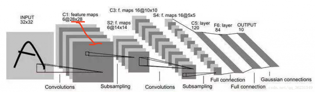
feather map的理解
在cnn的每个卷积层,数据都是以三维形式存在的。你可以把它看成许多个二维图片叠在一起(像豆腐皮一样),其中每一个称为一个feature map。
feather map 是怎么生成的?
输入层:在输入层,如果是灰度图片,那就只有一个feature map;如果是彩色图片,一般就是3个feature map(红绿蓝)。
其它层:层与层之间会有若干个卷积核(kernel)(也称为过滤器),上一层每个feature map跟每个卷积核做卷积,都会产生下一层的一个feature map,有N个卷积核,下层就会产生N个feather map。
卷积核的形状
每个卷积核具有长、宽、深三个维度。在CNN的一个卷积层中:
卷积核的长、宽都是人为指定的,长X宽也被称为卷积核的尺寸,常用的尺寸为3X3,5X5等;
卷积核的深度与当前图像的深度(feather map的张数)相同,所以指定卷积核时,只需指定其长和宽 两个参数。例如,在原始图像层 (输入层),如果图像是灰度图像,其feather map数量为1,则卷积核的深度也就是1;如果图像是grb图像,其feather map数量为3,则卷积核的深度也就是3.
卷积核个数的理解
该层卷积核的个数,有多少个卷积核,经过卷积就会产生多少个feature map,也就是下图中 豆腐皮儿的层数、同时也是下图豆腐块的深度(宽度)!!这个宽度可以手动指定,一般网络越深的地方这个值越大,因为随着网络的加深,feature map的长宽尺寸缩小,本卷积层的每个map提取的特征越具有代表性(精华部分),所以后一层卷积层需要增加feature map的数量,才能更充分的提取出前一层的特征,一般是成倍增加(不过具体论文会根据实验情况具体设置)
下面我们使用tensorflow 实现自定义的卷积核做简单的图片特征提取:
import os
os.environ['TF_CPP_MIN_LOG_LEVEL']='2'

import sys
sys.path.append('..')

from matplotlib import gridspec as gridspec
from matplotlib import pyplot as plt
import tensorflow as tf

import tensorflowTrain.sytleTransfer.kernels as kernels

def read_one_image(filename):
    ''' 从文件中读取图片,归一化处理并返回一个 tensor.
    '''
    #image_raw是bytes类型,还不是tensor
    image_raw = tf.gfile.FastGFile(filename, 'rb').read()
    #image_decoded是uint8类型的3阶Tensor
    image_decoded = tf.image.decode_jpeg(image_raw)

    #转换成float类型的tensor
    image = tf.cast(image_decoded, tf.float32) / 256.0
    return image

#使用各卷积核提取图片的特征,并把特征图片集合保存在数组images中
def convolve(image, kernels, rgb=True, strides=[1, 3, 3, 1], padding='SAME'):
    images = [image[0]]
    for i, kernel in enumerate(kernels):
        filtered_image = tf.nn.conv2d(image,
                                      kernel,
                                      strides=strides,
                                      padding=padding)[0]
        if i == 2:
            filtered_image = tf.minimum(tf.nn.relu(filtered_image), 255)
        images.append(filtered_image)
    return images

#显示核保存卷积核提取的feature map
def show_images(images, rgb=True):
    gs = gridspec.GridSpec(1, len(images))
    for i, image in enumerate(images):
        plt.subplot(gs[0, i])
        if rgb:
            plt.imshow(image)
        else:
            image = image.reshape(image.shape[0], image.shape[1])
            plt.imshow(image, cmap='gray')
        plt.axis('off')
    plt.show()


def main():
    rgb = False
    #不同的图片格式需要使用不同的卷积核集合
    if rgb:
        kernels_list = [kernels.BLUR_FILTER_RGB,
                        kernels.SHARPEN_FILTER_RGB,
                        kernels.EDGE_FILTER_RGB,
                        kernels.TOP_SOBEL_RGB,
                        kernels.EMBOSS_FILTER_RGB]
    else:
        kernels_list = [kernels.BLUR_FILTER,
                        kernels.SHARPEN_FILTER,
                        kernels.EDGE_FILTER,
                        kernels.TOP_SOBEL,
                        kernels.EMBOSS_FILTER]


    kernels_list = kernels_list[1:]
    #读取图片并把图片转换成float32型的tensor
    image = read_one_image('data/friday.jpg')
    #如果不是rgb图片,需要灰度处理图片
    if not rgb:
        image = tf.image.rgb_to_grayscale(image)

    #图片增加一个维度,变成只有1个元素的数组
    image = tf.expand_dims(image, 0) # make it into a batch of 1 element
    #对图片使用5个卷积核分别提取特征,生成的5个feature map保存在images List结构中
    images = convolve(image, kernels_list, rgb)

    #开始正式计算images数组中的 特征提取过程,并保存在images数组中
    with tf.Session() as sess:
        images = sess.run(images) # convert images from tensors to float values
    #显示特征图片
    show_images(images, rgb)

if __name__ == '__main__':
    main()
自定义卷积核:
import numpy as np
import tensorflow as tf

#都是4维数组
a = np.zeros([3, 3, 3, 3])
#a中第0阶为1,第1阶为1的所有值都赋值为0.25
a[1, 1, :, :] = 0.25
#a中第0阶为0,第1阶为1的所有值都赋值为0.125
a[0, 1, :, :] = 0.125
#a中第0阶为1,第1阶为0的所有值都赋值为0.125
a[1, 0, :, :] = 0.125
#a中第0阶为2,第1阶为1的所有值都赋值为0.125
a[2, 1, :, :] = 0.125
#a中第0阶为1,第1阶为2的所有值都赋值为0.125
a[1, 2, :, :] = 0.125
#a中第0阶为0,第1阶为0的所有值都赋值为0.0625
a[0, 0, :, :] = 0.0625
#a中第0阶为0,第1阶为2的所有值都赋值为0.0625
a[0, 2, :, :] = 0.0625
#a中第0阶为2,第1阶为0的所有值都赋值为0.0625
a[2, 0, :, :] = 0.0625
#a中第0阶为2,第1阶为2的所有值都赋值为0.0625
a[2, 2, :, :] = 0.0625

BLUR_FILTER_RGB = tf.constant(a, dtype=tf.float32)

a = np.zeros([3, 3, 1, 1])
a[1, 1, :, :] = 1.0
a[0, 1, :, :] = 1.0
a[1, 0, :, :] = 1.0
a[2, 1, :, :] = 1.0
a[1, 2, :, :] = 1.0
a[0, 0, :, :] = 1.0
a[0, 2, :, :] = 1.0
a[2, 0, :, :] = 1.0
a[2, 2, :, :] = 1.0
BLUR_FILTER = tf.constant(a, dtype=tf.float32)

a = np.zeros([3, 3, 3, 3])
a[1, 1, :, :] = 5
a[0, 1, :, :] = -1
a[1, 0, :, :] = -1
a[2, 1, :, :] = -1
a[1, 2, :, :] = -1

SHARPEN_FILTER_RGB = tf.constant(a, dtype=tf.float32)

a = np.zeros([3, 3, 1, 1])
a[1, 1, :, :] = 5
a[0, 1, :, :] = -1
a[1, 0, :, :] = -1
a[2, 1, :, :] = -1
a[1, 2, :, :] = -1

SHARPEN_FILTER = tf.constant(a, dtype=tf.float32)

EDGE_FILTER_RGB = tf.constant([
	[[[ -1., 0., 0.], [ 0., -1., 0.], [ 0., 0., -1.]],
        [[ -1., 0., 0.], [ 0., -1., 0.], [ 0., 0., -1.]],
        [[ -1., 0., 0.], [ 0., -1., 0.], [ 0., 0., -1.]]],
          [[[ -1., 0., 0.], [ 0., -1., 0.], [ 0., 0., -1.]],
	[[ 8., 0., 0.], [ 0., 8., 0.], [ 0., 0., 8.]],
	[[ -1., 0., 0.], [ 0., -1., 0.], [ 0., 0., -1.]]],
	[[[ -1., 0., 0.], [ 0., -1., 0.], [ 0., 0., -1.]],
	[[ -1., 0., 0.], [ 0., -1., 0.], [ 0., 0., -1.]],
	[[ -1., 0., 0.], [ 0., -1., 0.], [ 0., 0., -1.]]]
])

a = np.zeros([3, 3, 1, 1])
a[0, 1, :, :] = -1
a[1, 0, :, :] = -1
a[1, 2, :, :] = -1
a[2, 1, :, :] = -1
a[1, 1, :, :] = 4

EDGE_FILTER = tf.constant(a, dtype=tf.float32)

a = np.zeros([3, 3, 3, 3])
a[0, :, :, :] = 1
a[0, 1, :, :] = 2 # originally 2
a[2, :, :, :] = -1
a[2, 1, :, :] = -2

TOP_SOBEL_RGB = tf.constant(a, dtype=tf.float32)

a = np.zeros([3, 3, 1, 1])
a[0, :, :, :] = 1
a[0, 1, :, :] = 2 # originally 2
a[2, :, :, :] = -1
a[2, 1, :, :] = -2

TOP_SOBEL = tf.constant(a, dtype=tf.float32)

a = np.zeros([3, 3, 3, 3])
a[0, 0, :, :] = -2
a[0, 1, :, :] = -1
a[1, 0, :, :] = -1
a[1, 1, :, :] = 1
a[1, 2, :, :] = 1
a[2, 1, :, :] = 1
a[2, 2, :, :] = 2

EMBOSS_FILTER_RGB = tf.constant(a, dtype=tf.float32)

a = np.zeros([3, 3, 1, 1])
a[0, 0, :, :] = -2
a[0, 1, :, :] = -1
a[1, 0, :, :] = -1
a[1, 1, :, :] = 1
a[1, 2, :, :] = 1
a[2, 1, :, :] = 1
a[2, 2, :, :] = 2
EMBOSS_FILTER = tf.constant(a, dtype=tf.float32)
第一个卷积核的打印结果:
[[[[0.0625 0.0625 0.0625]
   [0.0625 0.0625 0.0625]
   [0.0625 0.0625 0.0625]]

  [[0.125  0.125  0.125 ]
   [0.125  0.125  0.125 ]
   [0.125  0.125  0.125 ]]

  [[0.0625 0.0625 0.0625]
   [0.0625 0.0625 0.0625]
   [0.0625 0.0625 0.0625]]]


 [[[0.125  0.125  0.125 ]
   [0.125  0.125  0.125 ]
   [0.125  0.125  0.125 ]]

  [[0.25   0.25   0.25  ]
   [0.25   0.25   0.25  ]
   [0.25   0.25   0.25  ]]

  [[0.125  0.125  0.125 ]
   [0.125  0.125  0.125 ]
   [0.125  0.125  0.125 ]]]
#########tensorflow 实践 –分布式训练 #########
TensorFlow,客户端会话联系主节点,实际工作由工作节点实现,每个工作节点占一台设备(TensorFlow具体计算硬件抽象,CPU或GPU)。单机模式,客户端、主节点、工作节点在同一台服务器。分布模式,可不同服务器。
运行中,主节点进程和工作接点进程通过接口通信
参数服务器:
当计算模型越来越大,模型的参数越来越多,多到模型参数的更新,一台机器的性能都不够时,我们需要将参数分开到不同的机器去存储和更新。参数服务器可以是多台机器组成的集群,类似于分布式的存储结构。主要用来解决参数存储和更新的性能问题
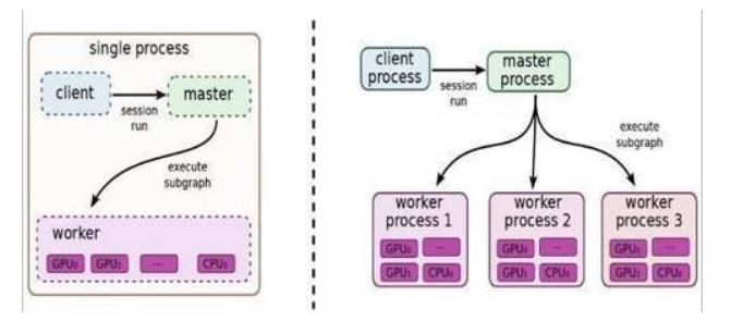
客户端基于TensorFlow的编程接口,构造计算图。此时,TensorFlow并未执行任何计算。直至建立会议会话,并以会议为桥梁,建立客户端与后端运行时的通道,将的Protobuf格式的GraphDef发送至分布式Master。也就是说,当客户对OP结果进行求值时,将触发Distributed Master的计算图的执行过程
分布式训练主要使用multiprocessing 库实现多进程
import tensorflow as tf
import multiprocessing as mp
import numpy as np
import os, shutil


TRAINING = True

# 构造数据集
x = np.linspace(-1, 1, 100)[:, np.newaxis]
noise = np.random.normal(0, 0.1, size=x.shape)
y = np.power(x, 2) + noise

#并发执行单元函数
def work(job_name, task_index, step, lock):
    #  设置 分布式环境集群节点信息: ip:port,
    cluster = tf.train.ClusterSpec({
        "ps": ['localhost:2221', ],#参数服务器
        "worker": ['localhost:2222', 'localhost:2223', 'localhost:2224',]
    })

    '''ClusterSpec的定义,需要把你要跑这个任务所有的ps和worker的节点的ip和端口信息都包含进去,所有的节点都要执行这段代码,大家就互相知道了,这个集群里都有哪些成员,不同成员的类型是什么,是ps节点还是worker节点
tf.train.Server定义开始,每个节点就不一样了。根据执行的命令参数不同,决定了这个任务是哪个任务。如果任务名字是ps的话,程序就join到这里,作为参数更新的服务,等待其他worker节点给他提交参数更新的数据。如果是worker任务,就继续执行后面的计算任务。
'''
    server = tf.train.Server(cluster, job_name=job_name, task_index=task_index)

    if job_name == 'ps':
        # 如果任务名字是ps的话,程序就join到这里,作为参数更新的服务,等待其他worker节点给他提交参数更新的数据
        print('Start Parameter Server: ', task_index)
        server.join()
    else:
        #worker 服务执行
        print('Start Worker: ', task_index, 'pid: ', mp.current_process().pid)

        '''replica_device_setter,在这个with语句之下定义的参数,会自动分配到参数服务器上去定义,如果有多个参数服务器,就轮流循环分配。
        '''
        with tf.device(tf.train.replica_device_setter(
                worker_device="/job:worker/task:%d" % task_index,
                cluster=cluster)):

            '''构建一个NN网络和计算逻辑
            '''
            tf_x = tf.placeholder(tf.float32, x.shape)
            tf_y = tf.placeholder(tf.float32, y.shape)
            l1 = tf.layers.dense(tf_x, 10, tf.nn.relu)
            output = tf.layers.dense(l1, 1)
            loss = tf.losses.mean_squared_error(tf_y, output)
            global_step = tf.train.get_or_create_global_step()
            train_op = tf.train.GradientDescentOptimizer(
                learning_rate=0.001).minimize(loss, global_step=global_step)

        # set training steps
        hooks = [tf.train.StopAtStepHook(last_step=100000)]

        # get session
        with tf.train.MonitoredTrainingSession(master=server.target,
is_chief=(task_index == 0),checkpoint_dir='./tmp', hooks=hooks) as mon_sess:
            print("Start Worker Session: ", task_index)
            while not mon_sess.should_stop():
                # train
                _, loss_ = mon_sess.run([train_op, loss], {tf_x: x, tf_y: y})
                with lock:
                    step.value += 1
                if step.value % 500 == 0:
                    print("Task: ", task_index, "| Step: ", step.value, "| Loss: ", loss_)
        print('Worker Done: ', task_index)


def parallel_train():
    if os.path.exists('./tmp'):
        shutil.rmtree('./tmp')
    #使用并发多进程创建本地集群1个参数服务和4个worker服务
    jobs = [('ps', 0), ('worker', 0), ('worker', 1), ('worker', 2)]
    step = mp.Value('i', 0)
    lock = mp.Lock()
    ps = [mp.Process(target=work, args=(j, i, step, lock), ) for j, i in jobs]
    [p.start() for p in ps]
    [p.join() for p in ps]


def eval():
    tf_x = tf.placeholder(tf.float32, [None, 1])
    l1 = tf.layers.dense(tf_x, 10, tf.nn.relu)
    output = tf.layers.dense(l1, 1)
    saver = tf.train.Saver()
    sess = tf.Session()
    saver.restore(sess, tf.train.latest_checkpoint('./tmp'))
    result = sess.run(output, {tf_x: x})
    # plot
    import matplotlib.pyplot as plt
    plt.scatter(x.ravel(), y, c='b')
    plt.plot(x.ravel(), result.ravel(), c='r')
    plt.show()


if __name__ == "__main__":
    if TRAINING:
        parallel_train()
    else:
        eval()
没有评论